World Health Sensor

Objective

Using The Global Health Observatory OData API to fetch data from it’s data collection. Analyze the data using data science techniques and create an interactive dashboard and deploying it using cloud services.

Project Tools

Data Source:

The Global Health Observatory https://www.who.int/data/gho
OData API documentation: https://www.who.int/data/gho/info/gho-odata-api

Retrieve the data:

requests to make HTTP requests to the OData API and retrieve the data.
Pandas: Perform data preprocessing, cleaning, filtering, and transformation using the powerful data manipulation capabilities of pandas.

Analyze the Data:

Pandas: Utilize pandas for exploratory data analysis (EDA), data wrangling, and statistical analysis on the retrieved data.
Stats: Module that contains correlation functions and statistical tests among other fuctions.

Visualization Tools:

Matplotlib: Create static visualizations such as line plots, bar charts, and scatter plots.
Seaborn: Build aesthetically pleasing and informative statistical visualizations.
Plotly: Develop interactive and customizable visualizations, including interactive charts and dashboards.

Design the Dashboard:

Dash: Useful to build interactive web-based dashboards using Python and HTML components.

Deploy the Dashboard:

AWS cloud services
TMUX library.

Test and Iterate:

User feedback and testing: Gather feedback from potential users and testers to improve the functionality and user experience of your dashboard.
Jupyter Notebook or documentation: Document the project, including the data analysis process, code, and key findings.

Project steps

Select the Data Source: Determine the specific API that provides the data needed for the analysis. Explore available public datasets. Determine the analysis goals.
Understand the API: Study the documentation of the OData API to understand its endpoints, query parameters, and how to retrieve data. Identify the available resources, data models, and relationships between entities.
Retrieve and Preprocess Data: Use the OData API to fetch the required data based on the analysis goals. Apply data preprocessing steps like cleaning, filtering, and transforming the data as necessary to prepare it for analysis.
Analyze the Data: Utilize data science techniques and libraries such as pandas, stats to perform exploratory data analysis (EDA), statistical analysis and visualizations. Extract meaningful insights and identify patterns or correlations in the data. Select the appropriate visualization tool like Matplotlib, Seaborn, or Plotly to create interactive and informative visualizations.
Design the application/dashboard: Design the user interface and layout of the dashboard using Dash library. Create an intuitive and user-friendly dashboard that allows users to interact with the visualizations, apply filters, and explore the data dynamically. Iterate on the design and make improvements based on user input and additional data analysis requirements.
Deploy the Dashboard: Host the dashboard on a web server or a cloud platform to make it accessible online. This involves deploying it as a web application utilizing AWS cloud hosting services. Test and Iterate: Test the functionality and usability of the dashboard, seeking feedback from potential users.

Select the Data Source

What I found exploring the GHO Data Collection:

The GHO data repository serves as the World Health Organization’s (WHO) portal to health-related statistics concerning its 194 Member States.
The Data could be explored by Theme, Category or Indicator.
The GHO data repository offers access to a wide range of health indicators, exceeding 2000 in number.
Indicators cover crucial health topics such as mortality, disease burden, Millennium Development Goals, non-communicable diseases, infectious diseases, health systems, environmental health, violence, injuries, and equity, among others.
Several indicators do not contain data or the data is not updated or completed.

Understanding the API

The Global Health Observatory (GHO) is constructed using a technology called RESTful web service. REST stands for Representational State Transfer, which is an architectural style used to design networked applications. In this context, GHO uses RESTful web services as the underlying technology to provide access to its data.

RESTful web services use standard HTTP methods (such as GET, POST, PUT, DELETE) to interact with resources (data) over the internet. These resources are identified by URLs, and the web service responds with data in a structured format, often in JSON or XML.

By using a RESTful web service, the Global Health Observatory can allow users to easily retrieve health-related data through standard web protocols, making it accessible and interoperable across various platforms and programming languages. This approach enables efficient data access and manipulation, making it convenient for data analysts and developers to fetch and utilize the health data provided by the GHO.

The documentation is clear and extensive.

Retrieve and Preprocess Data:

Use the OData API to fetch the required data based on the analysis goals. Apply data preprocessing steps like cleaning, filtering, and transforming the data as necessary to prepare it for analysis.

Retrieving

# Import the libraries

import pandas as pd
import requests
import json
import plotly.express as px
import matplotlib.pyplot as plt
import seaborn as sns
from scipy import stats

GET request to obtain the dimension data directly from the Global Health Observatory API

Retrieving all Dimension Values for Country dimension

# Send a GET request to the API endpoint
url = "https://ghoapi.azureedge.net/api/DIMENSION/COUNTRY/DimensionValues"
response = requests.get(url)

# Check the response status code
if response.status_code == 200:
    resp = response.json()
    data_countries = resp['value']
    # Process the data as needed
    for item in data_countries:
        value = item
    print('Request Successful')
        # Process each item in the data

else:
    print("Request failed with status code:", response.status_code)

Request Successful

# Create a countries DataFrame
countries = pd.DataFrame(data_countries)
countries.info()

<class 'pandas.core.frame.DataFrame'>
RangeIndex: 248 entries, 0 to 247
Data columns (total 6 columns):
 #   Column           Non-Null Count  Dtype 
---  ------           --------------  ----- 
 0   Code             248 non-null    object
 1   Title            248 non-null    object
 2   Dimension        248 non-null    object
 3   ParentDimension  242 non-null    object
 4   ParentCode       242 non-null    object
 5   ParentTitle      242 non-null    object
dtypes: object(6)
memory usage: 11.8+ KB

countries.head(5)

	Code	Title	Dimension	ParentDimension	ParentCode	ParentTitle
0	ABW	Aruba	COUNTRY	REGION	AMR	Americas
1	AFG	Afghanistan	COUNTRY	REGION	EMR	Eastern Mediterranean
2	AGO	Angola	COUNTRY	REGION	AFR	Africa
3	AIA	Anguilla	COUNTRY	REGION	AMR	Americas
4	ALB	Albania	COUNTRY	REGION	EUR	Europe

Retrieving all Indicators (list of indicators)

# Send a GET request to the API endpoint
url = "https://ghoapi.azureedge.net/api/Indicator"
response = requests.get(url)

# Check the response status code
if response.status_code == 200:
    resp = response.json()
    data_indicators = resp['value']
    # Process the data as needed
    for item in data_indicators:
        value = item
        value #print to see values
        # Process each item in the data

else:
    print("Request failed with status code:", response.status_code)

# Create a indicators DataFrame

indicators = pd.DataFrame(data_indicators)

indicators.info()

<class 'pandas.core.frame.DataFrame'>
RangeIndex: 2369 entries, 0 to 2368
Data columns (total 3 columns):
 #   Column         Non-Null Count  Dtype 
---  ------         --------------  ----- 
 0   IndicatorCode  2369 non-null   object
 1   IndicatorName  2369 non-null   object
 2   Language       2369 non-null   object
dtypes: object(3)
memory usage: 55.6+ KB

pd.set_option('display.max_colwidth', None)
indicators.sample(10)

	IndicatorCode	IndicatorName	Language
1295	SA_0000001512	Advertising restrictions at cinemas	EN
735	NCD_CCS_palliative_home	General availability of palliative care in community or home-based care in the public health system	EN
1333	SA_0000001534	On-premise sales restrictions on outlet density	EN
495	GOE_Q178	Individuals have the legal right to specify which health-related data from their EHR can be shared with health professionals of their choice	EN
1709	TOTENV_1	Deaths attributable to the environment	EN
638	MDG_0000000015	Prevalence of condom use by adults during higher-risk sex (15-49) (%)	EN
967	RADON_Q702	Mandatory mitigation measures if legal value is exceeded (existing buildings)	EN
1474	SA_0000001739_ARCHIVED	Alcohol, heavy episodic drinking (15+) past 30 days (%), age-standardized with 95%CI	EN
871	OCC_8	Occupational airborne particulates attributable DALYs per 100'000 capita	EN
470	GOE_Q138	Lack of suitable courses available	EN

The number of indicators is really high. Previous exploration of the data (directly in the website) showed that a lot of those indicators do not contain updated data or have several NaN values.

The API is working accordingly and I am pulling the data. Nevertheless the GHO website is not totally coherent with the list of indicators I am working with through the API. This add complexity to the process, considering it is relevant to find the indicator description. Additional description about it could be found in the extended version of this project.

Initially, I named the project the "World Health Sensor Project" because I aimed to work with reliable and comprehensive global health data. As I progressed, I narrowed my focus to tobacco-related data. However, the project has the potential for expansion to include analysis and communication of various other global health topics and indicators found in the GHO repository.

Retrieving Tobacco indicators

Tobacco use is indeed a significant contributor to a wide range of non-communicable diseases (NCDs) and is a leading cause of preventable illness and death worldwide. Non-communicable diseases are chronic conditions that are not caused by infectious agents but rather result from a combination of genetic, lifestyle, and environmental factors. These diseases include cardiovascular diseases (like heart disease and stroke), cancer, chronic respiratory diseases (such as chronic obstructive pulmonary disease), and diabetes. Division of Global Health Protection, Global Health, Centers for Disease Control and Prevention.

The harmful effects of tobacco use are primarily attributed to the various toxic substances present in tobacco products, such as nicotine, tar, and carbon monoxide. These substances can damage organs and tissues in the body and increase the risk of developing NCDs. It’s also worth noting that secondhand smoke exposure, which occurs when non-smokers breathe in smoke from tobacco products, is also harmful and can lead to similar health risks.

According with Canadian Cancer Society Second-hand smoke is what smokers breathe out and into the air. It’s also the smoke that comes from a burning cigarette, cigar or pipe. Second-hand smoke has the same chemicals in it as the tobacco smoke breathed in by a smoker. Hundreds of the chemicals in second-hand smoke are toxic. More than 70 of them have been shown to cause cancer in human studies or lab tests. Every year, about 800 Canadian non-smokers die from second-hand smoke.

# Looking for the indicators related with 'Tobacco'

Tobacco_indicators = indicators[indicators['IndicatorName'].str.contains('tobacco', case=False)]

Tobacco_indicators.sample(5)

	IndicatorCode	IndicatorName	Language
979	Rev_imp_other	Annual tax revenues - import duties and all other taxes (excluding corporate taxes on tobacco companies)	EN
2281	R_admin_tax_stamps_other	Tax stamps, fiscal marks, banderole or other types of marking are applied on other tobacco products	EN
1769	W14_harm_effects_C	Do health warnings on smokeless tobacco packaging describe the harmful effects of tobacco use on health?	EN
112	E12_compliance	Compliance of ban on brand name of non-tobacco products used for tobacco product	EN
1931	R_earmarking	Reported use of earmarked tobacco taxes	EN

The indicators related with Tobacco are divided by groups according with the strategy MPOWER. “These measures are intended to assist in the country-level implementation of effective interventions to reduce the demand for tobacco, contained in the WHO FCTC.” Read more clicking here

Tobacco_indicators.info()

<class 'pandas.core.frame.DataFrame'>
Int64Index: 137 entries, 47 to 2354
Data columns (total 3 columns):
 #   Column         Non-Null Count  Dtype 
---  ------         --------------  ----- 
 0   IndicatorCode  137 non-null    object
 1   IndicatorName  137 non-null    object
 2   Language       137 non-null    object
dtypes: object(3)
memory usage: 4.3+ KB

There are 137 indicators related with ‘Tobacco’, I’ll choose some on them to explore the data available

# Look for the MPOWER group indicators
MPOWER_indicators = Tobacco_indicators[Tobacco_indicators['IndicatorCode'].str.contains(r'^[A-Za-z]_Group', case=False)]
MPOWER_indicators

	IndicatorCode	IndicatorName	Language
104	E_Group	Enforcing bans on tobacco advertising, promotion and sponsorship	EN
615	M_Group	Monitoring tobacco use and prevention policies	EN
837	O_Group	Offering help to quit tobacco use	EN
881	P_Group	Protecting people from tobacco smoke	EN
935	R_Group	Raising taxes on tobacco	EN
1751	W_Group	Warning about the dangers of tobacco	EN

# Let's explore indicator related with prevalence

Tobacco_prevalence = Tobacco_indicators[Tobacco_indicators['IndicatorName'].str.contains('prevalence', case=False)]

Tobacco_prevalence

	IndicatorCode	IndicatorName	Language
614	M_Est_tob_curr	Estimate of current tobacco use prevalence (%)	EN
1942	Adult_curr_smokeless	Prevalence of current smokeless tobacco use among adults (%)	EN
2001	Yth_daily_smokeless	Prevalence of daily smokeless tobacco use among adolescents (%)	EN
2070	M_Est_smk_curr	Estimate of current tobacco smoking prevalence (%)	EN
2076	Adult_daily_smokeless	Prevalence of daily smokeless tobacco use among adults (%)	EN
2123	Yth_daily_tob_smoking	Prevalence of daily tobacco smoking among adolescents (%)	EN
2160	Adult_curr_tob_smoking	Prevalence of current tobacco smoking among adults (%)	EN
2163	Yth_curr_smokeless	Prevalence of current smokeless tobacco use among adolescents (%)	EN
2180	Adult_curr_tob_use	Prevalence of current tobacco use among adults (%)	EN
2256	Yth_curr_tob_use	Prevalence of current tobacco use among adolescents (%)	EN
2277	Yth_curr_tob_smoking	Prevalence of current tobacco smoking among adolescents (%)	EN
2311	M_Est_tob_curr_std	Estimate of current tobacco use prevalence (%) (age-standardized rate)	EN
2324	Adult_daily_tob_smoking	Prevalence of daily tobacco smoking among adults (%)	EN
2349	Adult_daily_tob_use	Prevalence of daily tobacco use among adults (%)	EN
2354	M_Est_smk_curr_std	Estimate of current tobacco smoking prevalence (%) (age-standardized rate)	EN

There are 15 indicators related with tobacco and prevalence.

I used a for loop to write the urls and explore the data in all the indicators within the word ‘Prevalence’, the process is available in the extended version on GitHub. Finally, the indicator I found more interesting by the amount of data it provides was M_Est_smk_curr_std == Estimate of current tobacco use prevalence (%)

Summarizing the indicators exploration:

Indicators to work with in the dashboard:

Indicator Code	Indicator Name
M_Est_smk_curr_std:	Estimate of current tobacco use prevalence (%)
M_Group:	Monitoring tobacco use and prevention policies
P_Group:	Protecting people from tobacco smoke
O_Group:	Offering help to quit tobacco use
W_Group:	Warning about the dangers of tobacco
E_Group:	Enforcing bans on tobacco advertising, promotion and sponsorship
R_Group:	Raising taxes on tobacco
NCD_UNDER70:	Premature deaths due to noncommunicable diseases (NCD) as a proportion of all NCD deaths

Indicators Dataframes

# Create a for loop to create the urls for the indicators I found interesting.

IndicatorCodes = ['M_Est_smk_curr_std', 'M_Group', 'P_Group', 'O_Group', 'W_Group', 'E_Group', 'R_Group', 'NCD_UNDER70']

urls = []

for Codes in IndicatorCodes:
    # Create the URLs
    url = f"https://ghoapi.azureedge.net/api/{Codes}"
    urls.append(url)
    
urls

['https://ghoapi.azureedge.net/api/M_Est_smk_curr_std',
 'https://ghoapi.azureedge.net/api/M_Group',
 'https://ghoapi.azureedge.net/api/P_Group',
 'https://ghoapi.azureedge.net/api/O_Group',
 'https://ghoapi.azureedge.net/api/W_Group',
 'https://ghoapi.azureedge.net/api/E_Group',
 'https://ghoapi.azureedge.net/api/R_Group',
 'https://ghoapi.azureedge.net/api/NCD_UNDER70']

# Create a for loop to retrieve the data and transform it into dataframes

df_dictionary = {}

for url in urls:
    response = requests.get(url)

    # Check the response status code
    if response.status_code == 200:
        resp = response.json()
        data = resp['value']            
        # Transform the json responses into dataframes.
        df = pd.DataFrame(data)  
        # Name the df with the indicator code 
        df_name = f"df_{url.split('/')[-1]}"
        # Include each name df into a dictionary
        df_dictionary[df_name] = df
        
    else:
        print("Request failed with status code:", response.status_code)

        # print the dictionary of dataframes.        
print(df_dictionary.keys())

dict_keys(['df_M_Est_smk_curr_std', 'df_M_Group', 'df_P_Group', 'df_O_Group', 'df_W_Group', 'df_E_Group', 'df_R_Group', 'df_NCD_UNDER70'])

# Extract the dfs from the dictionary

df_M_Est_smk_curr_std = df_dictionary['df_M_Est_smk_curr_std']
df_M_Group = df_dictionary['df_M_Group']
df_P_Group = df_dictionary['df_P_Group']
df_O_Group = df_dictionary['df_O_Group']
df_W_Group = df_dictionary['df_W_Group']
df_E_Group = df_dictionary['df_E_Group']
df_R_Group = df_dictionary['df_R_Group']
df_NCD_UNDER70 = df_dictionary['df_NCD_UNDER70']

# print the shape

for df in [df_M_Est_smk_curr_std, df_M_Group, df_P_Group, df_O_Group, df_W_Group, df_E_Group, df_R_Group, df_NCD_UNDER70]:
    print(f'{df.shape[0]} rows and {df.shape[1]} columns')

rows and 23 columns
rows and 23 columns
rows and 23 columns
rows and 23 columns
rows and 23 columns
rows and 23 columns
rows and 23 columns
rows and 23 columns

As df_R_Group has less rows than the other groups, after joining I’ll need to fill NaN values with zeros and make the notation is when displaying this data. Fortunately, the score goes from 1 to 6, then use 0 is not mislading.

Prepocessing

Keep just the columns of interest and renamed to better communication

Countries

# Countries dataframe
countries.head(2)

	Code	Title	Dimension	ParentDimension	ParentCode	ParentTitle
0	ABW	Aruba	COUNTRY	REGION	AMR	Americas
1	AFG	Afghanistan	COUNTRY	REGION	EMR	Eastern Mediterranean

# Rename the columns
countries.rename(columns = {'Code': 'Country Code', 'Title': 'Country', 'ParentTitle': 'WHO Region'}, inplace = True)

# Select specific columns using the .loc indexer
final_countries = countries.loc[:, ['Country Code', 'Country', 'WHO Region']]

# Sanity check
final_countries.head(3)

	Country Code	Country	WHO Region
0	ABW	Aruba	Americas
1	AFG	Afghanistan	Eastern Mediterranean
2	AGO	Angola	Africa

Estimate Average Smoking Prevalence

# Estimate of current tobacco use prevalence (%) dataframe
df_M_Est_smk_curr_std.head(1)

	Id	IndicatorCode	SpatialDimType	SpatialDim	TimeDimType	TimeDim	Dim1Type	Dim1	Dim2Type	Dim2	...	DataSourceDim	Value	NumericValue	Low	High	Comments	Date	TimeDimensionValue	TimeDimensionBegin	TimeDimensionEnd
0	27794728	M_Est_smk_curr_std	COUNTRY	DZA	YEAR	2020	SEX	BTSX	None	None	...	None	15.2	15.2	None	None	Projected from surveys completed prior to 2020.	2022-01-17T09:30:38.763+01:00	2020	2020-01-01T00:00:00+01:00	2020-12-31T00:00:00+01:00

1 rows × 23 columns

# Rename the columns
df_M_Est_smk_curr_std.rename(columns = {'SpatialDim': 'Country Code', 'ParentTitle': 'WHO Region', 'TimeDim' : 'Year', 'Dim1': 'Sex', 'Value': 'Prevalence'}, inplace = True)

# Select specific columns using the .loc indexer
final_prevalence = df_M_Est_smk_curr_std.loc[:, ['Country Code', 'Year', 'Sex', 'Prevalence']]

# Sanity check
final_prevalence.head(3)

	Country Code	Year	Sex	Prevalence
0	DZA	2020	BTSX	15.2
1	BEN	2020	BTSX	4.7
2	BWA	2020	BTSX	15

MPOWER indicators

# Rename the columns
df_M_Group.rename(columns = {'SpatialDim': 'Country Code', 'ParentTitle': 'WHO Region', 'TimeDim':'Year', 'Value': 'M_score'}, inplace = True)
df_P_Group.rename(columns = {'SpatialDim': 'Country Code', 'ParentTitle': 'WHO Region', 'TimeDim':'Year', 'Value': 'P_score'}, inplace = True)
df_O_Group.rename(columns = {'SpatialDim': 'Country Code', 'ParentTitle': 'WHO Region', 'TimeDim':'Year', 'Value': 'O_score'}, inplace = True)
df_W_Group.rename(columns = {'SpatialDim': 'Country Code', 'ParentTitle': 'WHO Region', 'TimeDim':'Year', 'Value': 'W_score'}, inplace = True)
df_E_Group.rename(columns = {'SpatialDim': 'Country Code', 'ParentTitle': 'WHO Region', 'TimeDim':'Year', 'Value': 'E_score'}, inplace = True)
df_R_Group.rename(columns = {'SpatialDim': 'Country Code', 'ParentTitle': 'WHO Region', 'TimeDim':'Year', 'Value': 'R_score'}, inplace = True)

# Select specific columns using the .loc indexer
final_M = df_M_Group.loc[:, ['Country Code', 'Year', 'M_score']]
final_P = df_P_Group.loc[:, ['Country Code', 'Year', 'P_score']]
final_O = df_O_Group.loc[:, ['Country Code', 'Year', 'O_score']]
final_W = df_W_Group.loc[:, ['Country Code', 'Year', 'W_score']]
final_E = df_E_Group.loc[:, ['Country Code', 'Year', 'E_score']]
final_R = df_R_Group.loc[:, ['Country Code', 'Year', 'R_score']]

Premature deaths due to noncommunicable diseases (NCD) as a proportion of all NCD deaths

# NDC: Noncommunicable diseases
df_NCD_UNDER70.head(1)

	Id	IndicatorCode	SpatialDimType	SpatialDim	TimeDimType	TimeDim	Dim1Type	Dim1	Dim2Type	Dim2	...	DataSourceDim	Value	NumericValue	Low	High	Comments	Date	TimeDimensionValue	TimeDimensionBegin	TimeDimensionEnd
0	25578824	NCD_UNDER70	COUNTRY	AFG	YEAR	2000	SEX	MLE	GHECAUSES	GHE060	...	None	72.8 [55.8-83.5]	72.78874	55.84165	83.46061	None	2021-03-10T15:22:19.27+01:00	2000	2000-01-01T00:00:00+01:00	2000-12-31T00:00:00+01:00

1 rows × 23 columns

# Rename the columns
df_NCD_UNDER70.rename(columns = {'SpatialDim': 'Country Code','TimeDim':'Year', 'Dim1':'Sex', 'NumericValue':'PrematureDeaths/NCD'}, inplace = True)

# Select specific columns using the .loc indexer
final_premature_deaths = df_NCD_UNDER70.loc[:, ['Country Code', 'Year', 'Sex', 'PrematureDeaths/NCD']]

# Sanity check
final_premature_deaths.head(3)

	Country Code	Year	Sex	PrematureDeaths/NCD
0	AFG	2000	MLE	72.78874
1	AFG	2001	MLE	72.56174
2	AFG	2002	MLE	72.96648

Merging dataframes

Now concatenate the dataframes, it would be great to build just 1 dataframe. However, having some columns with more and less data, concatenating all of them would get NaN values and not option to set correct datatypes.

# Merging the DataFrames: final_countries, final_prevalence, final_MPOWER, and final_premature_deaths.

final_prevalence = final_countries.merge(final_prevalence, on='Country Code', how='inner')
final_premature_deaths = final_countries.merge(final_premature_deaths, on=['Country Code'], how='inner')
final_MPOWER = final_countries.merge(final_M, on=['Country Code'], how='inner')
final_MPOWER = final_MPOWER.merge(final_P, on=['Country Code', 'Year'], how='inner')
final_MPOWER = final_MPOWER.merge(final_O, on=['Country Code', 'Year'], how='inner')
final_MPOWER = final_MPOWER.merge(final_W, on=['Country Code', 'Year'], how='inner')
final_MPOWER = final_MPOWER.merge(final_E, on=['Country Code', 'Year'], how='inner')
final_MPOWER = final_MPOWER.merge(final_R, on=['Country Code', 'Year'], how='outer')

final_MPOWER

	Country Code	Country	WHO Region	Year	M_score	P_score	O_score	W_score	E_score	R_score
0	AFG	Afghanistan	Eastern Mediterranean	2007	1	3	3	2	4	NaN
1	AFG	Afghanistan	Eastern Mediterranean	2008	1	3	3	2	4	2
2	AFG	Afghanistan	Eastern Mediterranean	2010	1	3	3	2	4	2
3	AFG	Afghanistan	Eastern Mediterranean	2012	1	3	3	2	4	2
4	AFG	Afghanistan	Eastern Mediterranean	2014	2	3	3	2	4	3
...	...	...	...	...	...	...	...	...	...	...
1555	ZWE	Zimbabwe	Africa	2012	1	3	3	2	2	3
1556	ZWE	Zimbabwe	Africa	2014	2	3	2	2	2	3
1557	ZWE	Zimbabwe	Africa	2016	2	3	4	2	2	3
1558	ZWE	Zimbabwe	Africa	2018	2	3	4	2	2	3
1559	ZWE	Zimbabwe	Africa	2020	1	3	4	2	2	3

1560 rows × 10 columns

# Check values in R_score:
final_MPOWER['R_score'].unique()

array([nan, '2', '3', '1', '4', '5', 'Not applicable'], dtype=object)

# Replace 'Not applicable' with '0' in 'R_score'
final_MPOWER['R_score'] = final_MPOWER['R_score'].replace('Not applicable', '0')

# Fill NaN values with '0'
final_MPOWER['R_score'] = final_MPOWER['R_score'].fillna('0')

# Sanity check
final_MPOWER['R_score'].unique()

array(['0', '2', '3', '1', '4', '5'], dtype=object)

final_prevalence

	Country Code	Country	WHO Region	Year	Sex	Prevalence
0	AFG	Afghanistan	Eastern Mediterranean	2020	BTSX	9.5
1	AFG	Afghanistan	Eastern Mediterranean	2020	MLE	16.7
2	AFG	Afghanistan	Eastern Mediterranean	2020	FMLE	2.2
3	AFG	Afghanistan	Eastern Mediterranean	2005	BTSX	17.1
4	AFG	Afghanistan	Eastern Mediterranean	2005	MLE	27.5
...	...	...	...	...	...	...
4423	ZWE	Zimbabwe	Africa	2025	FMLE	0.6
4424	ZWE	Zimbabwe	Africa	2000	BTSX	19.5
4425	ZWE	Zimbabwe	Africa	2000	MLE	36.1
4426	ZWE	Zimbabwe	Africa	2000	FMLE	2.9
4427	ZWE	Zimbabwe	Africa	2015	FMLE	1.2

4428 rows × 6 columns

# Check datatypes

final_prevalence.info()

final_premature_deaths.info()

final_MPOWER.info()

<class 'pandas.core.frame.DataFrame'>
Int64Index: 4428 entries, 0 to 4427
Data columns (total 6 columns):
 #   Column        Non-Null Count  Dtype 
---  ------        --------------  ----- 
 0   Country Code  4428 non-null   object
 1   Country       4428 non-null   object
 2   WHO Region    4428 non-null   object
 3   Year          4428 non-null   int64 
 4   Sex           4428 non-null   object
 5   Prevalence    4428 non-null   object
dtypes: int64(1), object(5)
memory usage: 242.2+ KB
<class 'pandas.core.frame.DataFrame'>
Int64Index: 10980 entries, 0 to 10979
Data columns (total 6 columns):
 #   Column               Non-Null Count  Dtype  
---  ------               --------------  -----  
 0   Country Code         10980 non-null  object 
 1   Country              10980 non-null  object 
 2   WHO Region           10980 non-null  object 
 3   Year                 10980 non-null  int64  
 4   Sex                  10980 non-null  object 
 5   PrematureDeaths/NCD  10980 non-null  float64
dtypes: float64(1), int64(1), object(4)
memory usage: 600.5+ KB
<class 'pandas.core.frame.DataFrame'>
Int64Index: 1560 entries, 0 to 1559
Data columns (total 10 columns):
 #   Column        Non-Null Count  Dtype 
---  ------        --------------  ----- 
 0   Country Code  1560 non-null   object
 1   Country       1560 non-null   object
 2   WHO Region    1560 non-null   object
 3   Year          1560 non-null   int64 
 4   M_score       1560 non-null   object
 5   P_score       1560 non-null   object
 6   O_score       1560 non-null   object
 7   W_score       1560 non-null   object
 8   E_score       1560 non-null   object
 9   R_score       1560 non-null   object
dtypes: int64(1), object(9)
memory usage: 134.1+ KB

# Fix datatypes in M_POWER dataframe

final_prevalence['Prevalence'] = final_prevalence['Prevalence'].astype(float)
final_MPOWER['M_score'] = final_MPOWER['M_score'].astype(int)
final_MPOWER['P_score'] = final_MPOWER['P_score'].astype(int)
final_MPOWER['O_score'] = final_MPOWER['O_score'].astype(int)
final_MPOWER['W_score'] = final_MPOWER['W_score'].astype(int)
final_MPOWER['E_score'] = final_MPOWER['E_score'].astype(int)
final_MPOWER['R_score'] = final_MPOWER['R_score'].astype(int)

# Sanity check

final_prevalence.info()
final_MPOWER.info()

<class 'pandas.core.frame.DataFrame'>
Int64Index: 4428 entries, 0 to 4427
Data columns (total 6 columns):
 #   Column        Non-Null Count  Dtype  
---  ------        --------------  -----  
 0   Country Code  4428 non-null   object 
 1   Country       4428 non-null   object 
 2   WHO Region    4428 non-null   object 
 3   Year          4428 non-null   int64  
 4   Sex           4428 non-null   object 
 5   Prevalence    4428 non-null   float64
dtypes: float64(1), int64(1), object(4)
memory usage: 242.2+ KB
<class 'pandas.core.frame.DataFrame'>
Int64Index: 1560 entries, 0 to 1559
Data columns (total 10 columns):
 #   Column        Non-Null Count  Dtype 
---  ------        --------------  ----- 
 0   Country Code  1560 non-null   object
 1   Country       1560 non-null   object
 2   WHO Region    1560 non-null   object
 3   Year          1560 non-null   int64 
 4   M_score       1560 non-null   int64 
 5   P_score       1560 non-null   int64 
 6   O_score       1560 non-null   int64 
 7   W_score       1560 non-null   int64 
 8   E_score       1560 non-null   int64 
 9   R_score       1560 non-null   int64 
dtypes: int64(7), object(3)
memory usage: 134.1+ KB

Great! Now is easier to deal with the data and build the graphs to the dashboard.

Visualizations

Note: Values from 2000 to 2018 are estimated based on national surveys. From 2020 to 2025 the values are projections.

This section includes some of the visualizations, if you want to see all of them you can explore the GitHub repository.

Estimate Average Smoking Prevalence by Sex over the time

# Group by Sex and Year and calculate the mean of Prevalence

average_numeric_value_over_years = final_prevalence.groupby(['Sex', 'Year'])['Prevalence'].mean().reset_index()

pivot_table = pd.pivot_table(
    average_numeric_value_over_years,
    values='Prevalence',
    index='Year',
    columns='Sex',
    aggfunc='mean'
)

pivot_table.reset_index(inplace=True)

fig = px.line(
    pivot_table,
    x='Year',
    y=pivot_table.columns[1:],  
    title='Estimate Average Smoking Prevalence by Sex over the time'
)

fig.update_layout(
    xaxis_title='Year',
    yaxis_title='Prevalence (%)',
)

fig.show()

Alt text

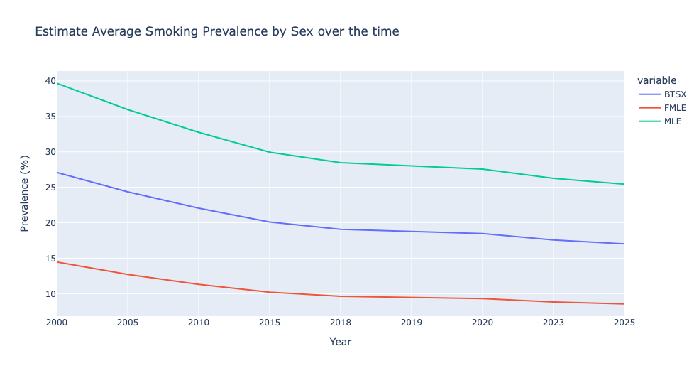
Estimate prevalence in males is ~3 times bigger than in females group.
The trend in the prevalence by sex groups is to decline. The prevalence projected by 2025 is ~15% lesss than the estimation in 2020. Females are expected to have a reduction of 6% in 2025.

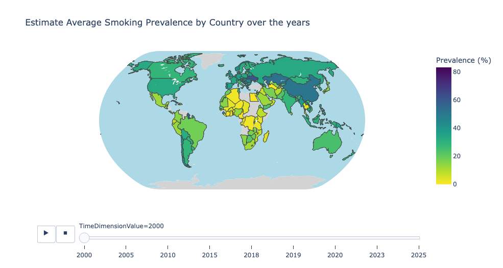
Estimate Average Smoking Prevalence by Country over the years

# Sort the dataframe by Year in ascending order
aggregated_data = final_prevalence.sort_values('Year')

fig = px.choropleth(
    aggregated_data,
    locations='Country',  
    locationmode='country names',  
    color='Prevalence',  
    hover_name='Country',  
    animation_frame='Year',  
    color_continuous_scale='Viridis_r', 
    title='Estimate Average Smoking Prevalence by Country over the years',
)

fig.update_geos(
    showcoastlines=True,
    coastlinecolor='RebeccaPurple',
    showland=True,
    landcolor='LightGrey',
    showocean=True,
    oceancolor='LightBlue',
    projection_type='natural earth',  
)

fig.update_layout(
    geo=dict(showframe=False, showcoastlines=False),
    coloraxis_colorbar=dict(title='Prevalence (%)'),
)

fig.show()

Alt text

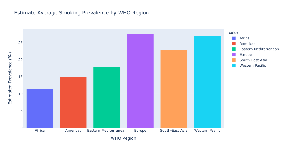
Estimate Average Smoking Prevalence by WHO Region

# Group by WHO Region and calculate the mean of Estimate Average Smoking Prevalence
average_numeric_value = final_prevalence.groupby('WHO Region')['Prevalence'].mean()

# Estimate Average Smoking Prevalence by WHO Region

fig = px.bar(
    x=average_numeric_value.index, 
    y=average_numeric_value.values,
    color=average_numeric_value.index,
    labels={'x': 'WHO Region', 'y': 'Estimated Prevalence'},
    title='Estimate Average Smoking Prevalence by WHO Region',
)

fig.update_layout(
    xaxis_title='WHO Region',
    yaxis_title='Estimated Prevalence (%)',
)

fig.show()

Alt text

Get country MPOWER data function

Writting a function to get the indicator value for each country:

def get_country_data(final_MPOWER, country):
    
    country_data = final_MPOWER[final_MPOWER['Country'] == country] 
    if country_data.empty:
        return f'wrong spelling or "No data available for {country}'  
    
    specific_data = country_data[['Country', 'Year', 'M_score', 'P_score', 'O_score', 'W_score', 'E_score', 'R_score' ]]

    return specific_data

result = get_country_data(final_MPOWER, 'Canada')
result

	Country	Year	M_score	P_score	O_score	W_score	E_score	R_score
232	Canada	2007	4	5	3	4	2	0
233	Canada	2008	4	5	5	4	2	4
234	Canada	2010	4	5	5	4	4	4
235	Canada	2012	4	5	5	5	4	4
236	Canada	2014	4	5	5	5	4	4
237	Canada	2016	4	5	5	5	4	4
238	Canada	2018	4	5	5	5	4	4
239	Canada	2020	4	5	5	5	4	4

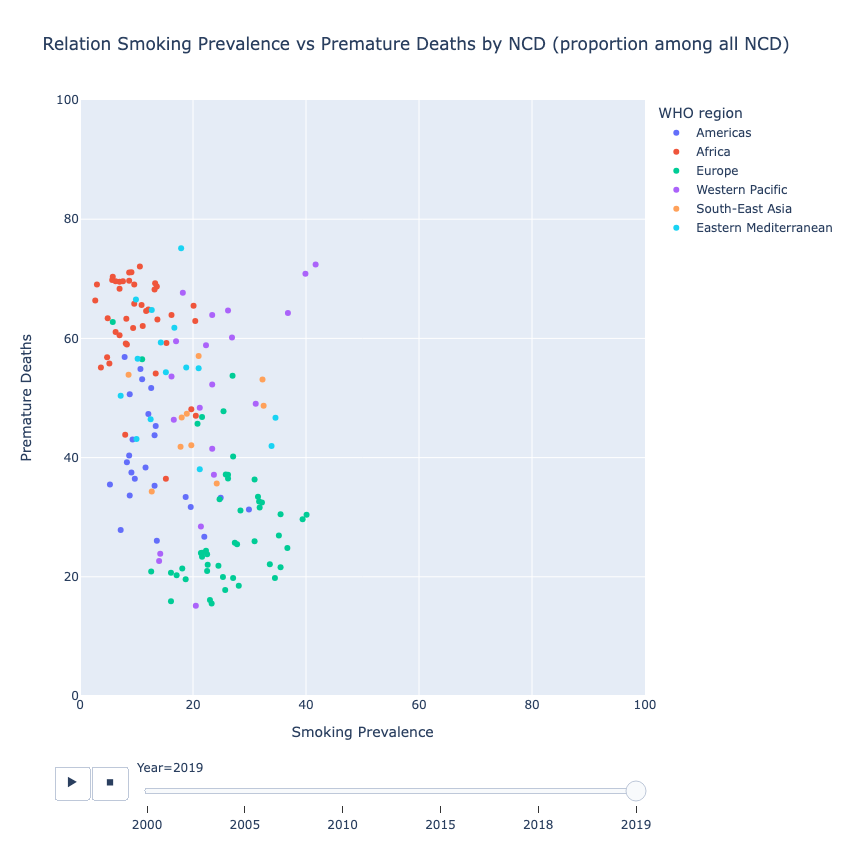
Relation Smoking Prevalence vs Premature Deaths by Noncommunicable Diseases (NDC) (proportion among all NCD)

# Merging data to the scatterplot 
scatter_data = pd.merge(final_prevalence, final_premature_deaths, on=['Country Code', 'Country', 'WHO Region', 'Year', 'Sex'])
scatter_data

	Country Code	Country	WHO Region	Year	Sex	Prevalence	PrematureDeaths/NCD
0	AFG	Afghanistan	Eastern Mediterranean	2005	BTSX	17.1	71.98372
1	AFG	Afghanistan	Eastern Mediterranean	2005	MLE	27.5	74.25545
2	AFG	Afghanistan	Eastern Mediterranean	2005	FMLE	6.7	69.67499
3	AFG	Afghanistan	Eastern Mediterranean	2010	BTSX	14.0	70.07750
4	AFG	Afghanistan	Eastern Mediterranean	2010	MLE	23.4	72.69907
...	...	...	...	...	...	...	...
2839	ZWE	Zimbabwe	Africa	2019	FMLE	0.9	56.25971
2840	ZWE	Zimbabwe	Africa	2000	BTSX	19.5	56.86102
2841	ZWE	Zimbabwe	Africa	2000	MLE	36.1	59.35542
2842	ZWE	Zimbabwe	Africa	2000	FMLE	2.9	54.56320
2843	ZWE	Zimbabwe	Africa	2015	FMLE	1.2	58.01034

2844 rows × 7 columns

Pearson Correlation Coefficient (Pearson’s r)

from scipy import stats

prevalence = scatter_data['Prevalence']
deaths = scatter_data['PrematureDeaths/NCD']

pearson_corr = stats.pearsonr(prevalence, deaths)
pearson_corr

PearsonRResult(statistic=-0.09868028979854496, pvalue=1.3413969700439424e-07)

The correlation between these two variables suggests a weak negative correlation statistically significant.

# Scatterplot of Smoking Prevalence vs Premature Deaths

fig = px.scatter(
    scatter_data,
    x='Prevalence',
    y='PrematureDeaths/NCD',
    title='Relation Smoking Prevalence vs Premature Deaths by NCD (proportion among all NCD)',
    labels={'Prevalence': 'Smoking Prevalence', 'PrematureDeaths/NCD': 'Premature Deaths'},
    animation_frame='Year',
    color = 'WHO Region',
    width=850, 
    height=850 
)

# Set fixed axis ranges
fig.update_xaxes(range=[0, 100])
fig.update_yaxes(range=[0, 100])

# Show the plot
fig.show()

Alt text

Design the Application/Dashboard

Now let’s write the csv files to work with them in the python script where the application is going to be defined.

# final_prevalence.to_csv('final_prevalence.csv')
# final_premature_deaths.to_csv('final_premature_deaths.csv')
# final_MPOWER.to_csv('final_MPOWER.csv')
# scatter_data.to_csv('scatter_data.csv')

I’m going to create a Python script for building the dashboard using the Dash framework.

I chose Dash for building the dashboard due to its seamless integration with Python and its ability to create interactive web applications for data visualization with relative ease. Dash’s Python-centric approach means I can leverage my existing Python programming skills without having to learn new languages. Its declarative syntax for defining the layout and interactions simplifies the development process. Additionally, Dash offers a wide range of pre-built components for creating charts, graphs, and interactive elements, reducing the need for extensive custom coding. The framework’s active community and extensive documentation provide a wealth of resources to troubleshoot issues and learn best practices. Overall, Dash’s combination of simplicity, versatility, and compatibility with Python makes it a powerful choice for rapidly developing engaging and interactive dashboards.

Overal Process View

First, I’ll make sure I have Dash installed. Then, I’ll set up my Python script, which I’ll name application.py, and import the necessary libraries. With the app initialized, I’ll define the layout using HTML and Dash components, structuring the interface the way I want it. To make the dashboard interactive, I’ll use callbacks that respond to user inputs and update the displayed content accordingly. Once everything is set up, I’ll run the app command and access it through my web browser. This process will allow me to create a dynamic and interactive dashboard for data visualization and analysis.

Dashboard description

As I explained, after connecting with GHO API, the exploration derived in the building of the dashboard: Global Tobacco Insights: Visualizing Smoking Trends, Health Consequences, and Control Policies a dashboard that display important information about Smoking Prevalence by sex, countries and WHO regions, the relationship between smoking rates and premature deaths caused by non-communicable diseases (NCDs), and the efforts being undertaken by the countries to accomplish the MPOWER strategy.

The dashboard provides insights into the challenges and successes of addressing smoking on a global scale. It highlights regions striving for improved public health and emphasizes the commitment of the global community to tackle this critical issue. Nevertheless, this project also underscored the need for additional data to gain a more comprehensive understanding of the smoking landscape. This is particularly critical given that the most recent data available from the Global Health Observatory (GHO) for constructing this project dates back to 2020.

Personal comment: The subjective perception doesn’t align with reality either, as it assumes that I live in a country with a low smoking prevalence. However, my personal experience contradicts this assumption, as I regularly encounter situations where I inhale secondhand smoke from individuals on the streets, which wouldn’t be expected in a country with such low prevalence and really good Scores in Protecting strategy. This situation prompts me to consider the possibility that we might not be accurately measuring the actual consumption rates and policies accomplishment. Absolutely, there is a clear need for more data and dedicated efforts to address this public health issue.

Deploy the Application/Dashboard

I’ll start by pushing my application.py script and all the project files to this repository. To ensure a clean and reproducible environment, I’ll include a requirements.txt file listing all the dependencies, including Dash and other libraries used in the project.

Next, I’ll utilize EC2 AWS instance to deploy the dashboard. I’ll create the instance and configure it to host the app.

Steps to deploy the dash application using EC2 AWS instance

Log in on AWS.
Select in Services: EC2
Launch a new instance and choose an Amazon Machine Image on your convenience, I chose a AMI and instance type with free tier because its capacity was enough for deploying my project.
If you have not connected before with AWS you will need to create the Key Pair.
When instance state be Running go to instance settings -> Security and change the include a new port. My case the new port was 8050 as that was the port dash used to deploy the app.
Connect to your instance using SSH protocol.
Install the require libraries in your instance.
Move your the files you require to run your app to your instance, I cloned the repository in my instance.
I had to include Flask in my .py script and modify the code to access Dash app using the external IP address or domain name of the EC2 instance.
Run the application in your instance.
In Instance Details you will find the Public IPv4 address, add :8050 to that address to see the application running.
Install TMUX library and Detach the dash session to keep the app running even when you disconnect from the instance.

Application link

Access the dashboard here

Sources

Acknowledgments

Dash Python User Guide: Dash is the original low-code framework for rapidly building data apps in Python. Learn more here
Dash Bootstrap Components: dash-bootstrap-components is a library of Bootstrap components for Plotly Dash, that makes it easier to build consistently styled apps with complex, responsive layouts. Learn more here
Rahul Agarwal How to Deploy a Streamlit App using an Amazon Free ec2 instance?

Carol Calderon

World Health Sensor

Objective

Project Tools

Project steps

Select the Data Source

Understanding the API

Retrieve and Preprocess Data:

Retrieving

Retrieving all Dimension Values for Country dimension

Retrieving all Indicators (list of indicators)

Retrieving Tobacco indicators

Summarizing the indicators exploration:

Indicators Dataframes

Prepocessing

Countries

Estimate Average Smoking Prevalence

MPOWER indicators

Premature deaths due to noncommunicable diseases (NCD) as a proportion of all NCD deaths

Merging dataframes

Visualizations

Design the Application/Dashboard

Dashboard description

Deploy the Application/Dashboard

Steps to deploy the dash application using EC2 AWS instance

Application link

Sources

Acknowledgments

Recent Articles